Linear Congruential Generators
Linear Congruential Generators (or LCGs in short) are algorithms that can be used to generate pseudo random numbers. To generate a random number with an LCG we need three discrete parameters and a starting value. The parameters are
- the modulus \(M\), with \(0 < M\),
- the multiplier \(A\), with \(0 < A < M\) and
- the increment \(C\), with \(0 \leq C < M\).
The starting value is usually denoted as \(X_{0}\) with \(0 \leq X_{0} < M\).
To now generate a new random number from a starting point \(X_{n}\) (for the sake of generality we set \(n = 0\)), we simply calculate
\[X_{n+1} = A * X_{n} + C \mod M \mathrm{.}\]
Since all values are discrete the result of the linear transformation \(R = A * X_{n} + C\) is again a discrete number. Through the modulo operation \(X_{n+1} = R \mod M\) we assert \(0 \leq X_{n+1} < M\).
A few examples
To get a feeling for this formula we choose a couple of parameters and see what we get for the output.
\(M = 9\), \(A = 2\), \(C = 0\), \(X_{0} = 1\)
These parameters generate the following sequence of numbers:
\[ 2, 4, 8, 7, 5, 1, 2, 4, 8, 7, 5, 1, 2, 4, 8, 7, 5, 1, 2, 4, \dots \]
We can see that it repeats itself very quickly. This is of course due to the small modulus we choose. Furthermore we can see that it does not cover all the values in the interval \(\left(0, M\right)\). If we now choose a starting value that is any number in the sequence above, we will obtain the same sequence again. So let’s choose a value that has not occurred yet.
\(M = 9\), \(A = 2\), \(C = 0\), \(X_{0} = 3\)
These parameters generate the following sequence of numbers:
\[6, 3, 6, 3, 6, 3, 6, 3, 6, 3, 6, 3, 6, 3, 6, 3, 6, 3, 6, 3, \dots\]
This sequence is even less random, as it only takes on the values \(3\) and \(6\). Now we have exhausted all values in \(\left(0, M\right)\).
We can already tell that to obtain truly randomly looking numbers, we need to pick a larger modulus.
\(M = 251\), \(A = 33\), \(C = 0\), \(X_{0} = 1\)
We obtain
\[33, 85, 44, 197, 226, 179, 134, 155, 95, 123, 43, 164, 141, 135, 188, 180, 167, 240, 139, 69, \dots\]
This appears to be a much better sequence. At first glance we can not spot repeating values and we are also unable to predict a successor to some value. The only obvious shortcoming is the small modulus. A modulus of \(M = 251\) causes the values to only be in the range \(\left( 0, M\right)\). After \(250\) numbers the values will definitely start repeating.
Testing for randomness
Our third example already makes it hard to tell if these numbers are good pseudo random numbers. But what makes a sequence of pseudo random numbers good? The German Bundesamt für Sicherheit in der Informationstechnik (BSI) recommends a series of statistical tests [2]. These tests look at the binary sequence of the random numbers.
The binary number sequence of example three would be \[ 00100001, 01010101, 00101100, 11000101, 11100010, 10110011, 10000110, \dots \]
To perform the following tests we take all binary numbers and concatenate them into a long string. This string is then truncated to be exactly \(20000\) bits long. This binary string is denoted \(b\), individual bits are denoted \(b_{i}\) (for the \(i\)th bit). \[ b = 00100001010101010010110011000101111000101011001110000110\dots \]
There are a total of five statistical tests recommended:
Monobit Test
We sum up all bits in the string \(b\).
\[ X_{b} = \sum_{i=1}^{i=20000} b_{i}\mathrm{.}\]
To pass the monobit test the result \(X_{b}\) has to fulfill \(9654 < X_{b} < 10346\). In words: the sequence is binary, made up of ones and zeros. Either appearance is equally probable (exactly \(0.5\)). Therefore we expect the roughly the same number of ones as we have zeros.
Poker Test
We divide the binary sequence into segments of four bits each, \[ 0010, 0001, 0101, 0101, 0010, 1100, 1100, 0101, 1110, 0010, 1011, \dots \] We can turn each segment into a four bit number between \(0\) to \(15\). There are exactly \(16\) different numbers. We now count the occurrence of each of these numbers, denoted \(s_{i}\) with \(i \in [0, 15]\). With this we calculate the sum \[X_{s} = \sum_{i=0}^{i=15} s_{i}^{2} - 5000\mathrm{.}\]
To pass the poker test we expect \(1.03 < X_{s} < 57.4\) for the result of the sum. This is in essence a \(\chi^{2}\)-test with 15 degrees of freedom.
Runs Test
We look at the binary sequence and count sequences of ones and zeros. In the sequence \[ 1, 0, 0, 1, 1, 1, 0, 1 \] we have three sequences of length \(1\) (the first \(1\) and the \(0\) and the \(1\) at the end), one sequence of length \(2\) (\(0, 0\)) and one sequence of length \(3\) (\(1, 1, 1\)). The occurrences of each length has to follow a distribution if the sequence is truly random. For a sequence of length \(20000\) this distribution is as follows.
| Sequence length | Occurrence interval |
|---|---|
| 1 | 2267-2733 |
| 2 | 1079-1421 |
| 3 | 502-748 |
| 4 | 233-402 |
| 5 | 90-223 |
| 6 and more | 90-233 |
Long Runs Test
The Long Runs Test is essentially the same as the runs test. In this we just see if there are sequences of length \(34\) or longer in the binary sequence. If there are the test has failed.
Autocorrelation Test
The Autocorrelation Test tests sub sequences of the original binary sequence and looks how much they depend on each other (or how “similar” they are).
An explanation
Let’s take the sequence \[ b = 0, 0, 1, 0, 0, 0, 0, 1, 0, 1, 0, 1, 0, 1, 0, 1, 0, 0, 1, 0, 1, 1, 0, 0, \dots \] and create from it two sub sequences of length \(10\). We let \(s_{i}\) be the sub sequence of length \(10\) that was created by removing the first \(i\) bits from the sequence \(b\) and then removing everything that makes \(s_{i}\) longer than length \(10\). \[s_{0} = 0, 0, 1, 0, 0, 0, 0, 1, 0, 1\] \[s_{1} = 0, 1, 0, 0, 0, 0, 1, 0, 1, 0\] The next step is to perform a bitwise XOR operation on the two sequences, \[s_{0 \oplus 1} = s_{0} \oplus s_{1} = 0, 1, 1, 0, 0, 0, 1, 1, 1, 1\] XOR is a logic operation with the following logic table \[0 \oplus 0 = 0\mathrm{,} \quad 0 \oplus 1 = 1\mathrm{,} \quad 1 \oplus 0 = 1\mathrm{,} \quad 1 \oplus 1 = 0\] Then the sum of \(b_{0 \oplus 1}\) is calculated. For a totally uncorrelated original binary sequence we expect a value of roughly \(5\) (half the length of the sub sequences).
The actual test
For the actual test the sequences are \(5000\) bits long. We take bits \(b_{i}\) from the original sequence \(b\) and calculate for \(n \in [1, 5000]\) \[X_{n} = \sum_{j=1}^{j=5000} b_{j} \oplus b_{j+n}\] The test has passed when \(2326 < X_{n} < 2674\) for each \(n\). To avoid confusion it should be noted that the test is only performed on the first \(10000\) bits of the original sequence.
Example plots
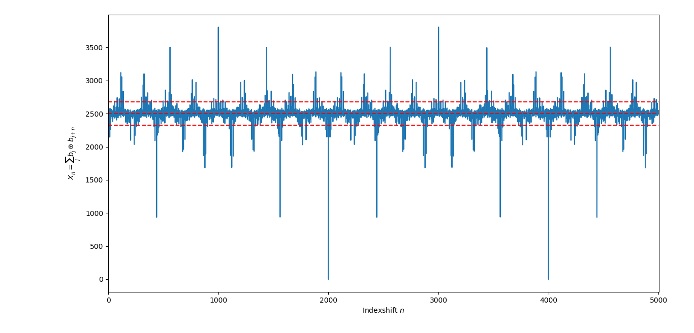
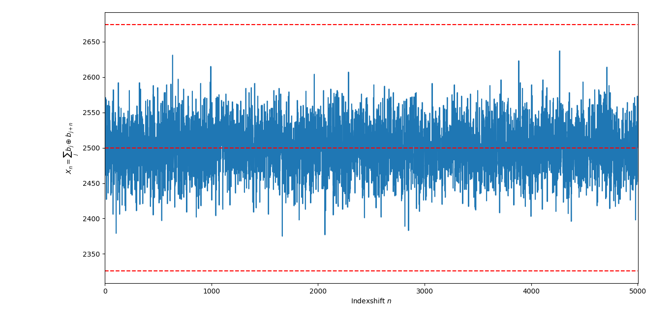
In the first image we can see the autocorrelation values of a binary sequence from an LCG where the modulus was choosen to be too small. The result is a strong autocorrelation. The second image shows the autocorrelation for a binary sequence that was generated by a quantum mechanical random number generator. Because of the quantum nature these numbers are truly random. This can also be seen in the autocorrelation plot.
Pitfalls of LCGs – The Spectral Test
Statistical tests are a good way of assessing some basic distribution properties of (pseudo random) binary sequences. In the case of pseudo random binary sequences generated from LCGs however, they don’t necessarily tell the whole story. Let’s generate a random number sequence \(X_{n}\) (the parameters for the LCG are \(X_{0} = 1\), \(A = 33\), \(C = 0\) and \(M = 251232131\); for these parameters all statistical tests pass) and look at the random number sequence \(X_{n}\) plotted against the random number sequence \(X_{n+1}\) (the same sequence, just shifted to the right by one number).
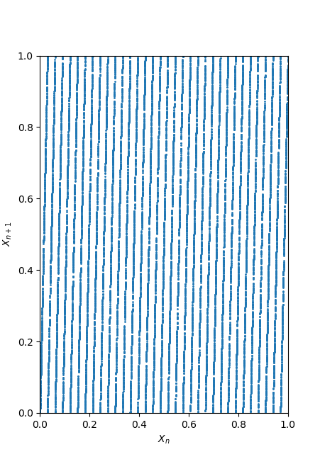
What do we see? Even though the statistical tests all pass, we see that the random numbers seem to fall onto a set of lines. We can find similar pictures in higher dimensions. For three dimensions we would have to plot \(X_{n}\) versus \(X_{n+1}\) versus \(X_{n+2}\). The random numbers would then fall on planes (or hyperplanes in four or more dimensions).
These lines are determined by our choice of parameters for the LCG. Since the increment \(C\) only shifts the random numbers it only affects the positions of the lines, not the distance or the angle. The distance and angle of the lines is determined by the multiplier \(A\) and the modulus \(M\).
The closer the lines are to each other, the higher quality the random numbers are. This is because a sequence of random numbers will fill the space (the squared interval \((0, M) \times (0, M)\) in two dimensions). This is what the Spectral Test does: it finds the distance (or rather the inverse of the distance) between adjacent lines (or (hyper-)planes).
For a detailed explanation please refer to the excellent (although technical) chapter on the Spectral Test in Knuths book [1] (pp. 89).
Performing the tests
To perform the tests that were introduced we can use the Python program downloadable here [3]. We pick a couple of “famous” LCG parameters and perform tests in a range around them.
RANDU
A very famous and bad example is the LCG implementation RANDU by IBM, that has been used since the 1960s [1]. The faults were discovered by 1963 but RANDU has been noted to have been in use up until 1999. RANDU is the reason that results from simulations from that era should always be taken with a grain of salt.
The parameters for RANDU are \[A = 65539\mathrm{,} \quad C = 0\mathrm{,} \quad M = 2^{31}-1\mathrm{.}\]
Statistical test
First we look at the statistical tests. Yellow colors indicate that all tests have passed. For the proposed parameter all statistical tests have passed. We notice a reduction in passed statistical tests for LCGs that have \(A = 65536 = 2^{16}\). We notice another reduction in passed tests when \(M\) changes from \(M = 2^{31} - 1\) to \(M = 2^{32}\). This is due to the padding of the generated bit sequence (going from \(31\) bits to \(32\) bits, while the first two bits will be equal to \(0\) most of the time. In general tests with even parameters \(A\) and \(M\) seem to fail more often.
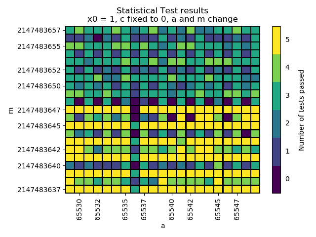
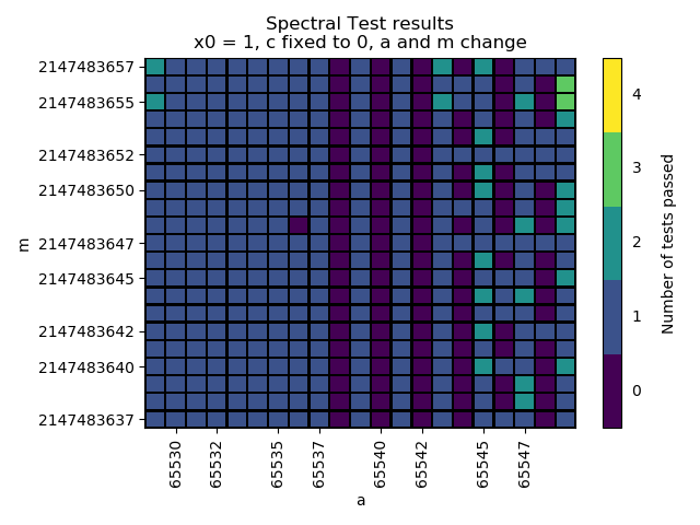
RANDU in an interval of \(A = 65539 \pm 10\) and \(M = (2^{31} - 1) \pm 10\).Spectral test
The Spectral Test is performed for the dimensions \(2\) to \(5\). These are still computationally easy. We note that for the chosen interval no parameter combination has passed the tests for every dimension \(2\), \(3\), \(4\) and \(5\). On the top right corner we spot two combinations that passed \(3\) out of \(4\) tests.
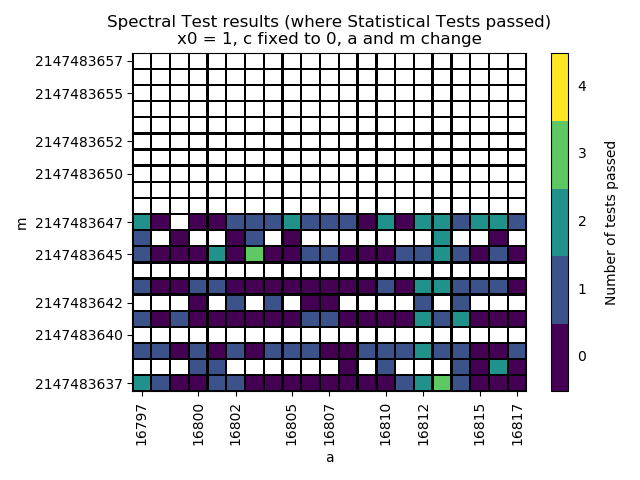
RANDU in an interval of \(A = 65539 \pm 10\) and \(M = (2^{31} - 1) \pm 10\).Spectral test when all statistical tests passed
Ideally the chosen parameters pass the statistical tests as well as the spectral test. For RANDU and the chosen interval around the proposed parameter combination, no combination passed all the statistical tests and the Spectral test for more than \(2\) dimensions.
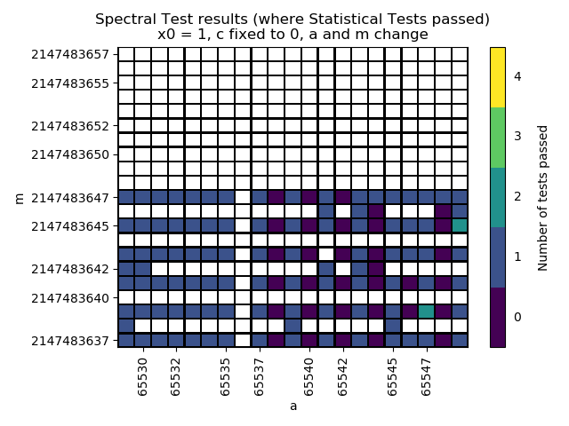
RANDU in an interval of \(A = 65539 \pm 10\) and \(M = (2^{31} - 1) \pm 10\). Parameters where the statistical tests failed are marked white.The conclusion is that RANDU is a very poor LCG and should not be used.
C++ LCG implementations
A more recent example is the LCG implementation found in the C++ standard [4]. There exist two different parameter choices, minstd_rand0 and minstd_rand.
minstd_rand0
minstd_rand0 has been adopted into the C++ “Minimal standard” in 1988. The parameters for minstd_rand0 are \[A = 16807\mathrm{,} \quad C = 0\mathrm{,} \quad M = 2^{31} - 1\mathrm{.}\]
Statistical test
We again notice a reduction in passed tests when \(M\) changes from \(M = 2^{31} - 1\) to \(M = 2^{32}\).
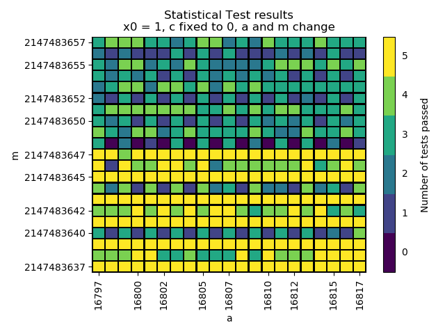
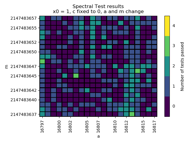
minstd_rand0 in an interval of \(A = 16807 \pm 10\) and \(M = (2^{31} - 1) \pm 10\).Spectral test
The results for the Spectral test for this version of the C++ LCG is comparable to the RANDU results. In the chosen interval no parameter combination passes the tests for every dimension. We spot a few combinations that pass \(3\) out of \(4\) tests.
minstd_rand0 in an interval of \(A = 16807 \pm 10\) and \(M = (2^{31} - 1) \pm 10\).Spectral test when all statistical tests passed
The combined result is that we can’t find any parameter combinations where statistical tests and spectral tests both pass in conjunction.
minstd_rand0 in an interval of \(A = 16807 \pm 10\) and \(M = (2^{31} - 1) \pm 10\). Parameters where the statistical tests failed are marked white.We conclude that this version of the C++ LCG, minstd_rand0, is a poor choice and should not be used.
minstd_rand (no \(0\) at the end)
minstd_rand has been adopted into the C++ “Minimal standard” in 1993. The parameters for minstd_rand are \[A = 48271\mathrm{,} \quad C = 0\mathrm{,} \quad M = 2^{31} - 1\mathrm{.}\]
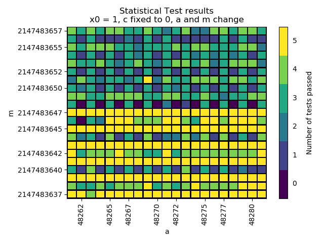
Statistical test
We again notice a reduction in passed tests when \(M\) changes from \(M = 2^{31} - 1\) to \(M = 2^{32}\). Other than that it compares well with the statistical test results from minstd_rand0.
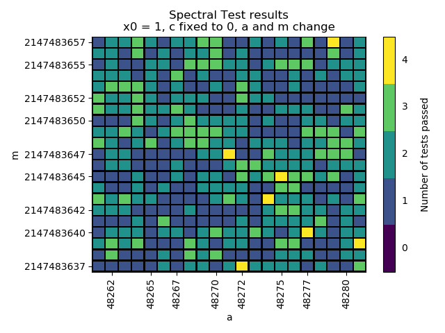
minstd_rand in an interval of \(A = 48271 \pm 10\) and \(M = (2^{31} - 1) \pm 10\).Spectral test
Comparing the results from the Spectral test for minstd_rand to minstd_rand0, minstd_rand looks a lot brighter. For the chosen interval we see \(7\) parameter sets that pass the Spectral test for every dimension. There are many parameter combinations for which \(3\) out of \(4\) tests pass.
minstd_rand in an interval of \(A = 48271 \pm 10\) and \(M = (2^{31} - 1) \pm 10\).Spectral test when all statistical tests passed
We finally see parameter combinations for which all statistical tests pass and for which then also the Spectral tests for every chosen dimension passes.
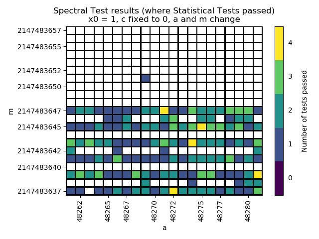
minstd_rand in an interval of \(A = 48271 \pm 10\) and \(M = (2^{31} - 1) \pm 10\). Parameters where the statistical tests failed are marked white.In the very center of the figure we see the proposed parameter for minstd_rand in yellow, meaning that it passed every statistical test and every Spectral test. We conclude that the proposed parameters are a reasonable choice.
Conclusion
We introduced a set of simple statistical tests [2] that can be used on random or pseudo random binary sequences. Additionally we implemented the Spectral test from [1]. They are fairly easy to implement and take about a second to complete on an average multicore computer.
Using these tests we looked at pseudo random numbers generated by LCGs for parameter combinations (and the combinations around it) that are commonly found. We discovered that some of the proposed parameters only pass the statistical tests. The Spectral test reveals that these parameter sets follow a structure that is not easily discovered by just looking at the statistical properties. Using pseudo random numbers generated by these LCGs in, for example, a Monte-Carlo simulation will likely lead to results that can not be trusted. The parameters proposed in the new “Minimal standard” in C++ appear to be a good choice. They pass all statistical tests introduced here, as well as the Spectral test up to dimension \(5\).
Further research is of course recommended.
References
- [1] Donald E. Knuth. The Art of Computer Programming, Volume 2: Seminumerical Algorithms. Addison-Wesley, 1997.
- [2] Werner Schindler. Functionality classes and evaluation methodology for deterministic random number generators. https://www.bsi.bund.de/SharedDocs/Downloads/DE/BSI/Zertifizierung/Interpretationen/AIS_20_Functionality_Classes_Evaluation_Methodology_DRNG_e.pdf, 1999.
- [3] Matthias Plock. lcg_tests. A small analysis suite for linear congruential generators for a university seminar. https://github.com/Klump3n/lcg_tests, 2019.
- [4] CPP Reference. std::linear_congruential_engine https://en.cppreference.com/w/cpp/numeric/random/linear_congruential_engine, looked up July 6, 2019.